WHY SHADING CALCULATIONS TAKE SO LONG
Calculating detailed solar shading and overshadowing is a problem for most building analysis tools, ECOTECT included. It is important to a whole range of building performance criteria, from thermal and daylighting analysis through to solar access and rights-to-light. However, doing it fully and properly can take a frustratingly long time. This article explains exactly what is happening during these calculations and offers tips on how to optimise the process and make best use of your existing shading data.
Introduction
When considering shading effects, two basic sources of both solar radiation and daylight must be considered. These are the Sun, which approximates a direct point source, and the entire sky dome, which approximates a diffuse hemispherical source. Things can get quite complicated because the Sun moves around quite a bit and the radiant distribution from the sky dome is often far from uniform.
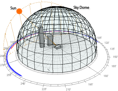
In theory, checking if any object is in shade at a particular time is simply a matter of determining if the Sun in it’s current position is obstructed by any other surrounding objects. In a computer model, this can be done by generating a ray from the object of interest in the direction of the Sun, and then checking if it intersects any other objects along it’s way.
This works if the object is a point, but if it’s a large surface it might be only partially in shade. It is possible to test for this by performing a full view factor calculation - extruding the surface towards the Sun and ‘clipping off’ the bits that are obstructed by other objects along the way. The fraction of the object exposed to the Sun at that time is found by dividing the surface area of the resulting shape by the full surface area of the object. The percentage in shade is then simply any fraction left over.
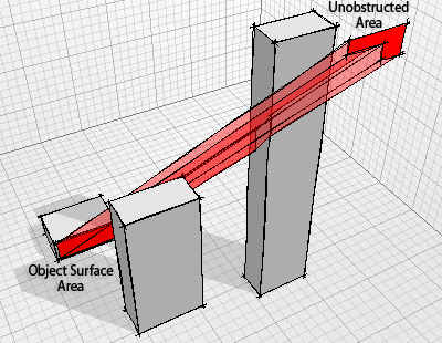
View factor calculations are quite involved, especially if the surrounding geometry is complex. Also, as the Sun moves around in the sky both hourly and seasonally, a separate calculation is required whenever the date and/or time changes. This makes using such detailed calculations pretty impractical and means that we have to look for ways to optimise the process without significantly compromising on accuracy.
Speeding Things Up
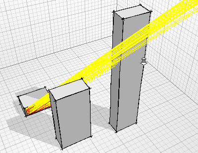
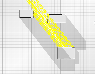
One way to speed things up is to use ray-tracing techniques instead of view factor calculations. This means generating a series of rays from sample points distributed over the surface we are interested in and checking each one for obstruction. The fraction of the surface exposed or in shade at any time is then calculated based on the number of rays obstructed compared to the total number that were generated.
Transparency and Reflection
Apart from being a bit quicker, this technique has some interesting additional benefits over the view factor method. Firstly, it can accommodate any number of transparent and/or translucent obstructions by multiplying the contribution of the ray by the fractional transmissivity of each such surface intersected. This way the ray only terminates when its contribution equals zero (ie: hits an opaque obstruction). Also whenever a shiny or reflective surface is intersected, it is possible to spawn additional reflected rays to see if the Sun ever bounces off that surface and reflects back onto the object being tested.
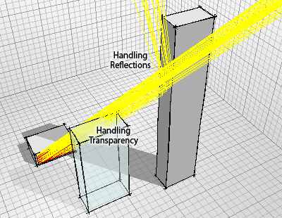
Shading Masks
Now, rather than having to recalculate these rays every time the date or time changes, it is possible to pre-calculate shading effects for many different parts of the sky. Ideally only those areas of the sky through which the Sun passes would need to be calculated. However, to accommodate the obstruction of diffuse radiation, check for all possible reflections and to allow maximum flexibility to consider different options, it is more practical to cover the entire sky dome.
By default ECOTECT divides the sky dome into 5 degree segments in both azimuth and altitude, however it is possible to set this as low as 2 degrees. As the Sun moves around, it is very quick to work out which sky segment it is in and then simply read off the shading data for that segment.
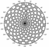
Plotted on sun-path diagram
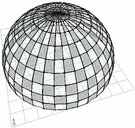
Plotted as 3D patches
A 5 degree by 5 degree spherical grid gives a total of 1296 segments (72 x 18), which is more than accurate enough for pretty well any application. A 2 degree by 2 degree spherical grid gives 8100 segments (180 x 45) which, though it might seem more accurate, really is overkill. In fact, the CIE recommend the use of only a total of 145 sky segments based on Tregenza’s early sky segmentation work (Tregenza, 1987). For more information, and to find out why equal-area subdivisions are not used, see the Square One wiki topic on Sky Subdivision.
Shading masks can be generated and stored for each surface in your ECOTECT model. When you perform a Calculate » Inter-Zonal Adjacency… calculation, ECOTECT automatically generates shading masks for each exposed surface on each thermal zone. These are stored in the model’s associated .shd file and used within the thermal analysis calculations, but you can also use them for incident solar radiation calculations and a range of other simulations. You can view and generate object shading masks at any time within the Calculate » Sun-Path Diagram… dialog box.
What Shading Masks Store
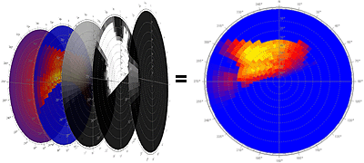
When calculating a shading mask, ECOTECT actually stores three layers of information for each segment:
shading from external obstructions,
angle of incidence effects (basically the cosine of the incidence angle to reduce the number of trigonometric call required) and
the fraction of radiation due to reflection off external obstructions back onto the object.
Each layer essentially acts as a filter. By loading a weather data file, it is possible to read hourly values for solar radiation and construct two additional layers for:
diffuse solar radiation and
direct solar radiation mapped over the same sky segments.
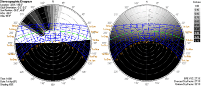
These last two layers represent cumulative sky distributions with different values generated in each segment based on the changing values of recorded direct solar radiation, the Sun position and the average radiant distribution of diffuse radiation.
When performing solar access calculations over a defined period, these sky distributions can be pre-calculated over the set date/time range - with the incidence, shading and reflections layers for each object in the study simply overlaid as needed to calculate the result.
Using Shading Masks in Calculations
Once you have all the data pre-calculated and stored in the different layers of each segment, calculations of solar access and incident radiation become relatively trivial. For each segment the diffuse and direct components are first added together to give the total cumulative radiation value. The reflected radiation effectively reduces the shading effect, so the shaded and reflected layers must then be added together. These two summed values, together with the incidence effect are then multiplied to give the total incident radiation in that segment.

Of course any combination of analysis can be done using only specific layers. For example, external shading, sunlight hours and sky factor calculations require only the shading and reflected layers. Sky components are a bit more complex in that they account for specific sky distributions and, in some cases, incidence effects. For more detailed information on the types of values that can be derived from shading masks, see the Square One wiki topic on Shading Mask Applications.

Obviously any calculations that deal with transmitted or absorbed solar radiation requires all five layers. However, the diffuse and direct cumulative skies need only be calculated once at the very beginning of each solar access analysis and stored as a global array. Only the incidence, shading and reflection layers are stored for each object.
The Effect of Model Changes
One of the most important aspects of using shading masks is that they only need to be recalculated when the physical geometry of the model or the transparency/reflectivity of any obstructions actually changes. This means that the same cached data can be used to compare variations in orientation, geographical location, solar access period and even entirely different hourly weather data files.
Shading masks are always calculated relative to model geometry. Changes in orientation or geographic location simply mean that the Sun travels through different sky segments at different times. Of course, when displayed in the Sun-Path Diagram, North is always shown vertically so it will look as if the masks themselves are rotating. However, in terms of the actual calculations, it is only the path of the Sun and, in the case of different weather data or solar access periods, only the direct and diffuse radiation layers that vary.

Getting the Best Results
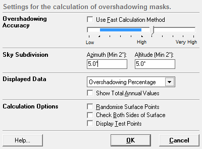
ECOTECT offers a number of settings for the calculation of shading masks. For detailed descriptions of each option it is obviously best to read the associated page in the help file, however there are some important concepts that might assist you get the best out of your shading mask calculations.
Using the Fast Calculation Method
In large models with many complex faces, it is often much quicker to generate an entire overshadowing diagram for each object than it is to trace a ray out to each of the 1296 sky segments. From the overshadowing diagram, individual pixels within each sky segment can be tested to see it they are part of the shaded or non-shaded areas. By sorting and generating shadow colours based on transparency, this method easily accommodates transparent and translucent obstructions, but cannot as yet deal with reflection effects.
As described in the Partial Shading topic on the Square One wiki, overshadowing diagrams are hard-edged, which means that any individual pixel will be either in shade or not. Thus, to determine the percentage shading for a surface, a separate overshadowing diagram is generated for each sampled point on the surface and the results then averaged for each sky segment.
On relatively small models with rectilinear geometry, the Fast Calculation Method is not necessary and can even be slower than the ray-tracing method. However, the complexity of the ray-tracing method increases almost exponentially with the number of obstructing objects in the model whereas the fast calculation method is much more linear. The graph in Figure 12 illustrates the relationship between the two.
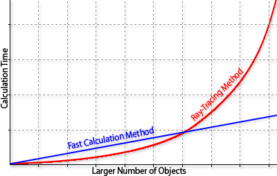
Obviously, if we could easily predict the intersection point between the two lines, we could have ECOTECT automatically choose the best one for each situation. Unfortunately this choice is a relatively complex function of the geometric complexity of each obstructing surface, the spatial relationship between objects in the model, the need to consider reflected radiation and the number of sky subdivisions used.
Overshadowing Accuracy
Overshadowing accuracy is one of the most important settings to get right. It basically controls the number of sample points used to calculate the partial shading of surfaces, varying from very low (a single point at the centre of the surface) to very high (a 100x100 grid giving a total of 100,000 points per surface). Obviously with so much variance, this value effectively determines how long each calculation will take.
When calculating shading masks for large obstructed surfaces, you will likely need to use medium-to-high accuracy (more points) to properly account for spatial variations in shading percentage. If the surface is not likely to be significantly overshadowed, you can get away with a relatively low accuracy.
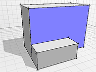
Sometimes it is necessary to break up a large surface into smaller segments in order to measure or visualise spatial variations in incidence. In these cases, it is important that you adjust the accuracy setting appropriately. For example, the situation in Figure 13 shows the application of the same accuracy setting before and after a large surface has been subdivided.
Single
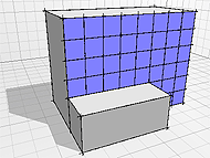
Multiple
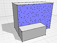
Single sampled
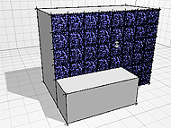
Multiple sampled
As you can see, the number of calculation points has increased enormously, but the result is unlikely to show a proportional increase in overall shading accuracy. As shown in Figure 14, the lowest possible accuracy setting is likely to be perfectly adequate for this situation.
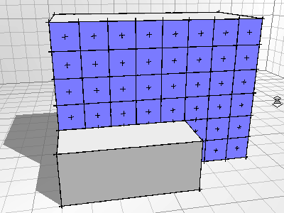
Thus the question of ‘how many points are necessary?’ is a difficult one. Typically, the area marked in blue within this setting’s slider is usually a good guide. Obviously if you have a lot of time to spare, tend towards the higher end of this blue region. If time is tight, tend towards the lower end.
Sky Subdivision
This setting determines the resolution of the spherical grid applied to the segmentation of the sky dome. Typically a 5 degree grid in both directions will be more than sufficient. Depending on the accuracy to which you have modelled the building geometry, rarely will a 2x2 degree grid give any greater accuracy - it may give slightly different results, but these may not be any closer to the ‘real’ situation than the 5x5 grid. In fact, for many early-stage design situations a 10x10 grid would be perfectly adequate.
Calculation Options
The most important setting here is the check both sides option. By default, ECOTECT only calculates shading for the side of the object in the direction of it’s surface normal. Anything behind the surface is ignored, effectively halving the calculation time and actually making it more accurate for thermal analysis. If you think about it, solar radiation entering though a window and hitting the back of an internal surface is an unnecessary complicating consideration as the heating effect of that radiation is already accounted for when the solar transmission through the window itself is calculated.
Having said that, sometimes it is useful to at least visualise the effects of radiation arriving on both sides as a surface, such as for a floor object that typically points downwards.
The second important calculation setting is the pseudo-random variation used when calculating sample point positions within each surface. Rather than use a uniform grid, ECOTECT applies a random jitter to each point equal in magnitude to half the grid size. This means that rows or columns of points don’t ‘just fit’ inside a linear edge, but some occur inside and some out based on the ratio of each grid square the surface occupies.
To get reproducible results, ECOTECT seeds the random number generator with the same start value at the beginning of each calculation. This means that running exactly the same calculation twice will give exactly the same results. If you choose this option, no random seed is used and the results of each calculation will be slightly different.
Finally, choosing to display test points can add visual interest to the calculation but, as the drawing canvas must be refreshed periodically (usually every 50 points), this can add substantially to the calculation time. Once you are comfortable with what these points are showing, it is best to leave this setting off.
Conclusion
Hopefully this explains at least to some degree the level of complexity required to properly account for overshadowing effects. ECOTECT’s use of multi-layered shading masks is quite revolutionary and the fact that it exposes much of their workings, allowing users to view, edit and manipulate them, makes this an extremely useful and flexible feature. However, even with the extensive optimisations used in their calculation, shading masks can take a long time to complete. Yet, once calculated properly, you can leverage and re-use them for a whole range of different types of analysis so its usually worth the wait.