CIE Sky Generator

Figure 1 - A screenshot of the CIE Sky app running within a web browser.

This web application lets you interactively experiment with the latest Perez All-Weather Sky model, which is the basis for the CIE Standard General Sky methodology described in both ISO 15469:2004(E) and CIE S 011/E:2003. This is basically a mathematical model for calculating representative spatial distributions of daylight over the sky dome that can functionally simulate a range of different weather conditions. Figure 2 shows some example real-world sky conditions and their modelled daylight distributions.

**Figure 2:** Some example real sky conditions and their modelled daylight distributions.

I use the term “latest Perez All-Weather Sky” model as the ISO and CIE standards are based on a more recent equation than the one included in Perez’s original paper and follow-up. I found this out the hard way whilst trying to validate the output of this tool against Radiance, DaySim, Honeybee and others. It turns out that these all implement the original Perez equations from 1993 instead of the more recent version updated in 1997 by Perez, Kittler and Durala, and adopted as the CIE standard in 2003. The differences are not huge, but enough to confound any direct comparison of results.

As a number of people have asked for more details about this, I wrote a blog post to explain. Also, I have written a much more detailed article on the process involved in calculating the Sky Distribution which better describes both the theoretical and algorithmic basis.

Getting Started

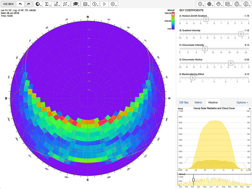
The calculated daylight distribution is governed by five (5) distinct sky coefficients. Whilst you can interactively manipulate any of these coefficients using the sliders provided, it is more typical for them to be automatically generated based on the type of sky being simulated or known weather conditions.

The CIE standard defines a set of 15 general sky types that represent different sky conditions - from overcast to cloudless and with varying levels of direct sunlight. An additional 16th type is given that is based on a much simpler mathematical model for overcast skies defined and used by CIE prior to this standard. Each sky type uses a specific configuration of these five coefficients. You can select any of these sky types using the list box adjacent to the coefficient sliders.

**Figure 3:** Examples of the 16 CIE standard general sky types.

The values for each sky coefficient can also be calculated from measured values of direct and diffuse illuminance and/or irradiance. Direct beam refers to sunlight coming directly from the Sun and its corona, as measured on a surface whose normal points directly at it. Diffuse horizontal refers to skylight coming from the rest of the sky dome as measured on a completely unobstructed horizontal surface.

You can set the direct and diffuse values using the interactive sliders in the Metric tab. Alternatively, once you have loaded some annual hourly weather data, you can select any date/time by pressing and dragging either chart in the Weather tab, or using the DATE AND TIME popover. Annual hourly weather data can also be used to simulate dynamic sky conditions at different times within the year or to generate a cumulative sky over any range of dates and times.

Sky Subdivision Type

The value calculated by the equations for any point in the sky is always given relative to the illuminance at the zenith of the sky dome. To convert these relative values to absolute values of illuminance or irradiance, it is necessary to normalise the total contribution of the whole sky so that it is equal to 1, and then multiply by the reference value of diffuse horizontal irradiance or illuminance. This typically means subdividing the sky dome into a series of discrete sky patches and then integrating all of their values to obtain the total contribution, taking care to properly account for Lambert’s cosine law and the area-weighting of each patch.

There are many ways to subdivide the sky dome into discreet patches. The simplest is to divide the sky into equal angle segments based on azimuth and altitude angles. This makes patch indexing very fast, but means that patches nearer the zenith are significantly smaller that those near the horizon. Another method is to vary the number of azimuthal patches in each altitudinal band in order to keep patch areas much more consistent in size. This makes patch indexing a bit trickier, but can be dealt with using iterators.

There are two variants of this method, one that divides the altitude into evenly distributed bands and calculates azimuthal patches as accurately as possible, and the other that leaves a single patch at the zenith and then uses various subdivisions of the 145 sky patches originally proposed by Tregenza. Figure 4 shows examples of the available subdivision methods.

Subdividing the sky based on equal-angle segments. — **Figure 4a:** Equal-angle sky subdivision.

Subdividing the sky based on equal-area segments. — **Figure 4b:** Equal-area sky subdivision.

Subdivision based on the Tregenza 145 patch sky. — **Figure 4c:** Subdivision using Tregenza's 145 patch sky.

Sky Subdivision Angle

Selecting an appropriate resolution for sky patches allows you to balance accuracy against calculation time. Whilst higher resolutions may increase overall accuracy, doubling the resolution also quadruples the required time. In many calculations the increase in accuracy due to increased patch resolution begins to fall away quite early whilst the calculation time increase is always exponential, so some experimental optimisation is usually necessary. Figure 5 shows some examples of sky distributions at different resolutions.

**Figure 5a:** Subdivision based on 15° segments.

**Figure 5b:** Subdivision based on 5° segments.

**Figure 5c:** Subdivision based on 2.5° segments.

**Figure 5d:** Subdivision based on 1.2° segments.

When the Reinhart/Tregenza subdivision method is selected, the available resolutions are based on integer subdivisions of each of the original 145 patches rather than azimuthal angle. Thus, dividing each original patch by 2 in each dimension gives 580 patches, by 3 gives 1305, by 4 gives 2320 and by 6 gives 5220.

Cumulative Sky Calculation

In many calculations it can be much more efficient to generate a single sky distribution that is the cumulative sum of many sequential instantaneous sky distributions, and then use that in the calculation once rather than running the calculation many times on multiple instantaneous skies.

Once you have annual hourly weather data loaded, you can use the Calculate Cumulative Sky… item in the Solar Analysis menu to do this. As shown in Figure 6, the dialog box allows you to select the type of metric to calculate, the components to include, the date/time range over which to aggregate values and the sub-hourly time step.

The options for generating cumulative sky distributions. — **Figure 6a:** Options for generating a cumulative sky.

The cumulative direct and diffuse components. — **Figure 6b:** Cumulative sky showing direct and diffuse.

Cumulative sky showing only diffuse component. — **Figure 6c:** Cumulative sky showing only diffuse.

Cumulative sky showing only direct component. — **Figure 6d:** Cumulative sky showing only direct.

Settings

The app provides a range of options and settings for the display and generation of sky distributions. Figure 7 shows some of the the popovers that allow you to select and/or change those values.

Options for adjusting the displayed colour scale. — **Figure 7a:** Tools for adjusting the colour scale.

Options for showing radiance or luminance, and direct sunlight. — **Figure 7b:** Showing radiance/luminance and sunlight.

Selecting the required subdivision and angular resolution. — **Figure 7c:** Subdivision type and angle resolution.

Sun-path components to display and projection methods. — **Figure 7d:** Sun-path components and projections.

**Figure 7e:** Setting the date and time of year.

Setting the geographic location of the site. — **Figure 7f:** Setting the geographic location.

Background

I developed this app as part of some work on a series of daylight and solar analysis tools, primarily to help me visually verify and debug my implementation of the CIE standard. The other key aim was to understand just how smoothly the model transitions between sky types when iterating through time using actual measured hourly weather data. It has already provided me with several useful insights that have helped significantly refine the process of interpolating between skies and aggregating at sub-hourly time intervals.

Change Log

0.0.1 2018-09-25

Initial release.

< PREV SOFTWARE: Schedule Editor NEXT: Psychrometric Chart SOFTWARE >