Making a Thermal Comparison

Introduction

The main purpose of simulation is to model as close as possible a real-world physical process. To be useful it is obviously important that simulation results closely match those from physical measurements taken in a similar actual situation. However, it is also important for you to first ensure that what is being calculated and what is being measured are actually comparable.

The most obvious comparison is between measured internal air temperatures and simulated temperatures within the same zone of a building. This is useful as air temperature is one of the major factors affecting the perception of comfort in any space, and it is relatively easy to both measure and predict. However, there are a number of important issues that throw into question whether the two values you get are directly comparable.

This is not to say that such a comparison is not valuable, but you must understand that you are probably not comparing the same thing in each case so there will be some fundamental and inherent differences.

Physical Location

Measured values from thermal sensors or thermometers are invariably taken at very specific locations within each space. Simulated zone temperatures on the other hand almost invariably represent the spatial average over the entire zone.

In real rooms you get localised heat spots and stratified air layers wherein those nearer the ceiling are warmer than those nearer the floor. Similarly, pockets of air near a cold window surface will be cooler and more subject to movement than the rest of the air closer to the centre of the room. There are a whole range of reasons why temperatures may vary significantly at different points in a zone.

These include:

• drafts of outside air that affect only certain areas,

• differential surface temperatures – due to highly conductive materials (glass, for example) or highly absorptive materials (exposed masonary or concrete) – which can result in localised radiant temperature issues or convective currents that induce localised air movement,

• heat plumes from equipment and even people,

• directional radiation from a radiant heater, and

• areas of direct sunlight that move across a space, etc.

Thus, it is quite possible that you will be physically measuring with your sensor one of these very localised effects – and you really have no way of knowing if this is the case.

Obviously if you stand next to the sensor you can easily detect significant drafts, but with clothes protecting most areas of your skin you may not be sensitive to lesser air movements and subtle radiant effects. More often though, individual sensors are left unattended for long periods so you really will have no idea what happened to them at different times.

It is possible to construct a very thorough model that can simulate many of these complex effects, but it requires huge attention to detail and analysis that involves iterating many times between a thermal solution and a computational fluid dynamics (CFD) run. Both are needed to accurately resolve the effects of air movement and surface radiation, but this is a difficult and time consuming process and one that defeats the purpose of a conceptual analysis to direct early decision-making.

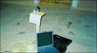
The best you can really do is use a large number of sensors in each space. You cannot reliably use one sensor and simply move it around as many of these localised effects are highly dynamic, potentiallty changing even as you are in the process of moving the sensor.

Radiant Effects

Even with a well protected sensor, it is very difficult to fully exclude radiant effects from other surfaces in the room when trying to measure air temperature. If you are close to a window, for example, it’s surface temperature is likely to be very different from the wall immediately adjacent. Being a physical object, the sensor will exchange energy with the window, either loosing heat if the window is cooler or gaining heat if it is significantly hotter.

The accurate calculation of localised radiant temperates is highly dependant on the geometry of each space and relatively time-intensive. Thus, most thermal analysis tools only calculate a mean radiant temperature (MRT) value which, once again, is averaged over the entire zone. In almost all cases the MRT assumes the room is a cube and that the sensor point is at its centre. This way it is based on the area weighted average of all surface temperatures – something that is quick to calculate and a very useful indication of the average radiant effect. However, it is not an accurate value for any specific location within the zone.

Some thermal analysis tools can calculate radiant temperatures at specific points, but you must specifically set up the calculation to do so and manually locate each point of interest. If you can get this information for your particular sensor location, and you know how to calculate the sensitivity of your sensor to radiant gains, then you can correct the measured temperature for radiant effects. However, to do this you have to assume that your thermal simulation is accurate in the first place in order to use it’s radiant temperatures so the comparison is somewhat compromised.

Measurement Error

In all temperature sensors there are inherent error margins in the values they record. These stem from the way each type of sensor converts a physical characteristic into an electrical signal. For example, some sensors use a small thermocouple which changes its electrical resistance with temperature. Others use metal springs whose coil tensions change or fluid solutions that change volume. All need to ensure that there is adequate air movement over the sensor itself whilst still providing physical protection against damage and radiant effects.

Most types of sensor also require callibration. Two sensors of exactly the same type located immediately adjacent to each other can give quite different recordings. It is standard practice to bring all your sensors together prior to a monitoring project and run them for several days to compare their measurements – the experience of the author is that differences in the order of 2°C are not uncommon.

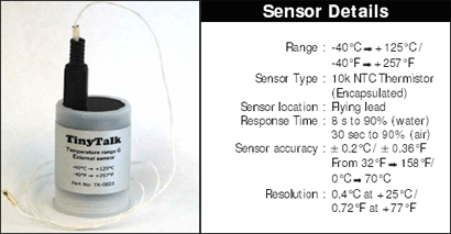
Whilst the accuracy of the enclosed sensor itself is not in question, many quoting error margins as low as ± 0.2°C, the absolute relationship between outside conditions and internal recording can be subject to some level of drift that needs to be corrected for with each sensor.

Accurate Weather Data

The next issue is whether the simulation is based on the exact same weather conditions experienced by the building being measured. As the calculated thermal response of any building is almost totally governed by external conditions, any meaningful comparison requires directly comparable weather data.

Portable weather stations that also accurately record both direct and diffuse solar data can be quite expensive. Thus it is not always possible to get good, reliable on-site weather data for the duration of the measurement period – you will most likely have to rely on recordings from the closest government weather station.

When using weather data from a remote weather station, it is virtually impossible to consider in the simulation model many of the micro-climate effects that may be impacting on the actual building. For example, hourly wind speeds at each window are not typically measured, so the simulation is usually based on measured wind speeds at the weather station, usually located on top of an unobstructed pole 6m in the air severa miles away – hardly the same conditions.

The Solution

All of the above considerations are true of any simulation comparison, and will always result in some variation between measured and simulated results. Whilst an understanding of the reasons for these differences allows you to factor in error margins, it is likely that these will be at least 3-5°C, making any precise comparison of absolute values rather questionable.

However, even though the actual temperatures themselves may not be directly comparable, what you should really be looking for are commonalities in the trends and fluctuations in each data set. If both the measured and simulated buildings respond similarly to a rapid rise in direct solar gains, or to the sudden ignition of an internal heat source, then you can have confidence in the relative accuracy of the comparison.

Assessing Relative Accuracy

The issue with relative accuracy is that you must have some reference against which to compare your new results. If you are simply testing a design, you can set up a base model and then compare any changes when different design options are applied. As long as you are only varying a small number of parameters at once, then you can be reasonably sure that you are observing their relative effect on the thermal conditions of each zone.

If you are comparing only measured and simulated datasets, establishing a reference is more difficult. In this case, you wiil have to use more complex statistical analysis.

We recently engaged in research for the AuditAC project which requires the calibration of simulation methods against extensive recorded data. As our methodologies progress, expect a series of follow-up articles outlining our approach to this whole topic.

Weaknesses

Obviously the inability to directly compare simulated and measured data significantly affects confidence in simulation results and the tools that produce them. It makes it much harder to trust that some anomolies have not crept in and, if they have, difficult to isolate what they are and why they are there.

Considering relative accuracy alone is good in that it keeps you heading in the right direction, but does not give you the absolute surety you may need to convince a client that your passive building will always work…

Conclusion

In most simulation work it is nearly always the relative accuracy of the modelling algorithm that is of most benefit. If the simulation system’s response to change is proportional to that of the real system, then it is a very useful tool for comparing design options.