RADIANCE AND DAYLIGHT FACTORS
The freely available RADIANCE software is one of only a few lighting analysis tools able to accurately calculate illuminance levels on surfaces within a building model. This article explains how illuminance levels can be used to generate daylight factors in RADIANCE and presents a number of ways of doing this, including using ECOTECT as a modelling interface. It also shows how both illuminance levels and daylight factors calculated in RADIANCE can be read back and displayed interactively within your ECOTECT model.
Introduction
The RADIANCE lighting simulation software from Lawrence Berkeley Laboratories [1] is currently the most accurate tool available for both daylighting and artificial lighting analysis. It uses a two-pass, hybrid, backwards-raytracing algorithm that can handle complex geometry and sophisticated material definitions. Moreover, it is one of only a few analysis tools that can calculate illuminance levels.

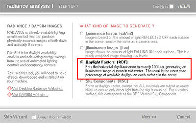
Like most lighting tools, RADIANCE defaults to generating luminance images. These are the same as we perceive when looking at a scene or when using a camera. Luminance is based on the amount of light reflected off objects, so such images display the colour and reflectance of each visible surface. The measure of luminance is the cd/m2 or its imperial equivalent the Nit. For a more detailed description of lighting units, see the Square One wiki topic on Light Measurements.
RADIANCE can also generate illuminance images. These are based on the amount of light falling on objects and therefore does not represent surface colours and reflectances - though light levels on each surface are affected by the colour and reflectance of the surfaces that surround them. Illuminance values are displayed in __Lux __and are usually much more important to a designer as almost all building regulations and international standards specify the minimum Lux values required for different environments and the tasks undertaken within them.
Lighting Calculations
RADIANCE works by resolving the radiant exchange of energy between light sources and surfaces within the model by dividing each surface into a series of sample points and generating spherical rays from each point to determine which other surfaces, light sources or sky sections are 'visible' from that point. It does this iteratively, continuously calculating and updating the estimated light levels at each point on each surface until a minimal difference threshold is met. This process establishes the spatial distribution of ambient light levels within the model, from which it can generate any number of forward ray-traced images as set up by the user.


Sky Illuminance & Daylight Factors
Illuminance levels deal with the actual amount of light hitting a surface and are therefore significantly affected by variations in the amount of light given off by the sky. Sky luminance is, in turn, affected by the position of the Sun as well as the amount, location and opacity of clouds within the visible sky dome. This makes it highly variable - sometimes changing quite substantially in a matter of only a few minutes.
To deal with these highly variable sky conditions, many building codes and design briefs use daylight factors as the design criteria instead of illuminance on the working plane. Daylight factors are expressed as the percentage of natural light falling on a work surface compared to that which would have fallen on a completely unobstructed horizontal surface under exactly the same sky conditions. Thus, a daylight factor of 5% on an internal surface means that it received only 1/20th of the maximum available natural light.
Converting surface illuminances to daylight factors is relatively easy in RADIANCE, but requires a couple of steps that can be a bit confusing.
Daylight Factors in Radiance
The simplest way to generate daylight factors in RADIANCE is to set the total horizontal illuminance of the generated sky to a known value, and then simply scale the calculated surface illuminances as a percentage of that total value.
It is possible to quantify the available light output of the whole sky by simply measuring the amount of light falling on a completely unobstructed horizontal surface. This measurement gives the total horizontal illuminance of the sky, which you can actually set in RADIANCE using the -B parameter to the gensky command. This parameter must be given as a radiant energy value in Watts per meter squared (W/m2).
Setting the Sky Horizontal Illuminance to 100
Obviously, if you set the total horizontal illuminance of the sky to be exactly 100, then you don’t have to do any scaling as the results will already be equivalent to a percentage. This is exactly what ECOTECT does when you select the Daylight Factor image type in the RADIANCE Export dialog.
As illuminance levels are given in Lux, you need to convert them to an equivalent radiant energy value in W/m2. As 1 Lux = 1 Lumen/m2, and RADIANCE uses a default luminous efficacy for daylight of 179 Lumens/Watt, this is done by dividing the total horizontal illuminance value required by 179 to give W/m2.
Thus, to generate an overcast sky with a total horizontal illuminance value of 100 Lux, ECOTECT sets the -B parameter to 0.558659 (100/179) by including a line similar to the following in the sky definition:
!gensky 4 1 12.00 -c -a -32.0 -o 116.0 -m 120.0 -B 0.558659
The initial three numbers give the month, day and time whilst the -a, -o and -m parameters refer to the current location’s latitude, longitude and timezone reference longitude respectively.
Important Note:
This method is fine when you are using RADIANCE with ECOTECT and
RadianceCP
as they will automatically set all the right scales and legend titles for you. However, in the RADIANCE calculation it will simply think you want a particularly dull sky. Thus, if you use only the image display tools that comes with RADIANCE (winimage.exe or ximage) to generate false-colour or iso-contoured images, they will still use the word ‘Lux’ at the top of the scale as it only really understands illuminance.
You can solve this problem by using RadianceIV the image tool that comes with ECOTECT to generate the images and enter the right units or, as a last resort, a quick touchup of the resulting image in your favourite image editing software.
Determining the Design Sky Illuminance
If you do not specify the total horizontal illuminance of the sky, RADIANCE will automatically calculate it based on the current date, time and model latitude. If you know what value was used by RADIANCE to generate any illuminance image, you can scale the resulting surfaces illuminances to a percentage and obtain your daylight factors that way.
The RadianceCP utility that comes with ECOTECT allows you to access this value by automatically creating a simple model comprising only a flat horizontal surface and the same sky conditions as specified in the scene you just exported. You can then use the trace command in the interactive image generator to display the lux level in the middle of this surface.

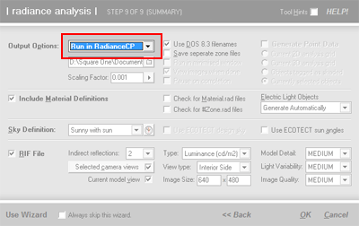
When you export your model to RADIANCE, choose the Run RadianceCP option in the Action selector. This will save your scene files and automatically load them in RadianceCP. If you then set the Image Type option to Daylight Factor in the Post Processing section, it will automatically apply a scaling factor and add the correct ‘DF’ title to the displayed scale.
When prompted during the main RadianceCP image calculation, simply enter this value into the displayed dialog and it will automatically work out the scaling factor based on the horizontal sky illuminance.
RadianceCP will then invoke the RADIANCE falsecolor utility within the batch file to filter and scale the original image from illuminance levels to daylight factors, adding a line similar to the following:
falsecolor -ip original.pic -s 15 -l DF -cl -m 0.254621 > dayfactor.pic
The -ip specifies the input picture, -s the maximum scale value, -l the legend title, -cl the generation of contour lines and -m the actual multiplier to use.
Grid Point Illuminances
Instead of displaying daylight factors only within the still images generated by RADIANCE, it is possible to import spatial point values back into ECOTECT directly from the RADIANCE scene files. This is done using the RADIANCE rtrace utility and requires a file containing the points at which these values are to be derived.
Exporting Grid Point Values
If you have the analysis grid displayed in ECOTECT when you export your model and choose the Final Render item in the Action selector of the RADIANCE Export Dialog, the Generate Point Data option will be available. If you check this and choose one the 2D option, a file will be generated containing all the currently visible analysis grid nodes. This file will be created with the same name as the exported Radiance scene, but with a .pts extension.

Each line in the .pts file contains 6 floating point values - the first three being the x, y and z coordinates of the grid point in model co-ordinates and the last three being the x, y and z vector values of the required surface normal at that point - indicating the direction the point is ‘facing’. ECOTECT will automatically invoke rtrace to process this file once the required images have been calculated and all the ambient data generated.
Importing Grid Point Values
During this calculation, a further file with the same name but with a .dat file extension will be created by RADIANCE containing all the radiant energy values at each point. ECOTECT will spawn a separate program thread to monitor and wait for this calculation to complete before prompting you to import back the calculated values. Depending on the complexity of your model, these calculations can take anywhere from 1 minute to several days, depending on the complexity of the model, so be prepared for a bit of a wait. During this wait you will have to keep the same model open ready to receive the new data. A useful trick is to simply start a new instance of ECOTECT in order to continue working.

The resulting .dat file contains three values per line, being the red, green and blue radiant energy values for each point, in the same order and on the same lines as points in the .pts file. When importing these, ECOTECT again assumes a luminous efficacy of 179 lumens/Watt in order to convert the radiant energy to an illuminance.
At the moment ECOTECT uses the positive direction of the currently selected analysis grid axis as the surface normal for each grid point. Whilst it is relatively easy to change this by simply replacing all the ‘1.000’ normal values with ‘-1.000’ using the find/replace function in your favourite text editor, the next version of ECOTECT will include a setting to allow this to be specified by the user.
As an alternate, there are scripts on the Square One website that demonstrate how it is possible to access selected objects in the model and generate .pts files from their centre points - as well as manually reading back in .dat files and assigning the values as object attributes. These allow almost limitless flexibility in the specification of points and surface normals.
Conclusion
Daylight factors are an important means of both specifying and comparing the daylighting performance of a building. The ability to generate daylight factors easily using ECOTECT and RADIANCE allows you to take advantage of the accuracy and complexity of RADIANCE’s lighting algorithms whilst displaying in ECOTECT exactly the data you need in the way that you need it.
References
- The Radiance Synthetic Imaging System
Lawrence Berkeley National Laboratories, Berkeley, California.
http://radsite.lbl.gov/radiance/